Equal Earth Documentation¶

Equal Earth Projection¶

This is a matplotlib add-on that adds the Equal Earth Projection described by Bojan Šavrič (@BojanSavric), Tom Patterson and Bernhard Jenny:

Abstract:: “The Equal Earth map projection is a new equal-area pseudocylindrical projection for world maps. It is inspired by the widely used Robinson projection, but unlike the Robinson projection, retains the relative size of areas. The projection equations are simple to implement and fast to evaluate. Continental outlines are shown in a visually pleasing and balanced way.”

This projection is similar to the Eckert IV equal area projection, but is 2-5x faster to calculate. It is based on code from:

https://matplotlib.org/gallery/misc/custom_projection.html

as well as code from @mbostock:

https://beta.observablehq.com/@mbostock/equal-earth-projection

Requirements¶

shapefile (from pyshp) is required to read the map data. This is available from Anaconda, but must be installed first, from the command line:

>>>conda install shapefile

Installation¶

Only the EqualEarth.py file is required. You can download the entire repository using the green “Clone or download” button, or by clicking on the file link, then right-clicking on the “Raw” tab to download the actual script. The script must be located in a directory in your PYTHONPATH list to use it in another program.

Note

Using the GeoAxes.DrawCoastline() (new in 2.0) function will create a maps folder in the same directory and download some maps (500kb) for drawing, the first time it is called.

New in This Version (2.0)¶

GeoAxes.DrawCoastlines():

World map data from Natural Earth will download into the maps folder in the same directory as the Equal Earth module, the first time this function is called. This is 500kb on disk, but is downloaded in .zip format and unzipped automatically. Other maps can be used if you supply the shape files. Once the axes is set up, you can draw the continents:

>>>ax.DrawCoastlines(facecolor='grey', edgecolor='k', lw=.5)

GeoAxes.plot_geodesic() Great Circle (geodesic) lines:

Navigation lines can be plotted using the shortest path on the globe. These lines take plot keywords and wrap around if necessary:

>>>pts = np.array([[-150, 45], [150, 45]])
>>>ax.plot_geodesic(pts, 'b:', linewidth=1, alpha=.8)

GeoAxes.DrawTissot():

Draw the Tissot Indicatrix of Distortion on the projection. This is a set of circles of equal size drawn on the projection, showing how the projection distorts objects at various positions on the map:

>>>ax.DrawTissot(width=10.)

See the Wikipedia article for more information.

Usage¶

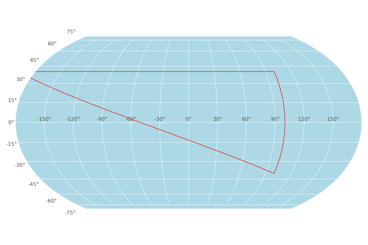
Importing the module causes the Equal Earth projection to be registered with Matplotlib so that it can be used when creating a subplot:

import matplotlib.pyplot as plt
import EqualEarth
longs = [-200, 100, 100, -200]
lats = [40, 40, -40, 40]
fig = plt.figure('Equal Earth Projection')
ax = fig.add_subplot(111, projection='equal_earth', facecolor='lightblue')
ax.plot(longs, lats)
plt.grid(True)
plt.tight_layout()
plt.show()

Note

ax.plot():

Lines drawn by ax.plot() method are clipped by the projection if any portions are outside it due to points being greater than +/- 180° in longitude. If you want to show lines wrapping around, they must be drawn twice. The second time will require the outside points put back into the correct range by adding or subtracting 360 as required.

Note that the default behaviour is to take all data in degrees. If radians are preferred, use the rad=True optional keyword in fig.add_subplot(), ie:

ax = fig.add_subplot(111, projection='equal_earth', rad=True)

All plots must be done in radians at this point.

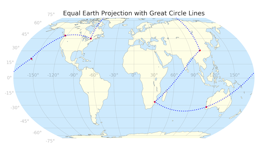
This example creates a projection map with coastlines using the default settings, and adds a few shortest-path lines that demonstrate the wrap-around capabilities:

import matplotlib.pyplot as plt
import EqualEarth
fig = plt.figure('Equal Earth', figsize=(10., 6.))
fig.clear()
ax = fig.add_subplot(111, projection='equal_earth',
                     facecolor='#CEEAFD')
ax.tick_params(labelcolor=(0,0,0,.25))  # make alpha .25 to lighten
pts = np.array([[-75, 45],
                [-123, 49],
                [-158, 21],
                [116, -32],
                [32.5, -26],
                [105, 30.5],
                [-75, 45]])
ax.DrawCoastlines(zorder=0)  # put land under grid
ax.plot(pts[:,0], pts[:,1], 'ro', markersize=4)
ax.plot_geodesic(pts, 'b:', lw=2)
ax.grid(color='grey', lw=.25)
ax.set_title('Equal Earth Projection with Great Circle Lines',
             size='x-large')
plt.tight_layout()  # make most use of available space
plt.show()

Future¶

Ultimately, the Equal Earth projection should be added to the cartopy module, which provides a far greater range of features.

@Author: Dan Neuman (@dan613)

@Version: 2.0

@Date: 13 Sep 2018

EqualEarth API¶

class EqualEarth.EqualEarthAxes(*args, rad=False, **kwargs)[source]¶

A custom class for the Equal Earth projection, an equal-area map projection, based on the GeoAxes base class.

https://www.researchgate.net/publication/326879978_The_Equal_Earth_map_projection

In general, you will not need to call any of these methods. Loading the module will register the projection with matplotlib so that it may be called using:

>>>import matplotlib.pyplot as plt
>>>import EqualEarth
>>>fig = plt.figure('Equal Earth Projection')
>>>ax = fig.add_subplot(111, projection='equal_earth')

There are useful functions from the base GeoAxes class, specifically:

GeoAxes.DrawCoastlines()

GeoAxes.plot_geodesic(), and

GeoAxes.DrawTissot()

GeoAxes.DrawShapes() can also be useful to draw shapes if you provide a shapefile:

>>>import shapefile
>>>sf = shapefile.Reader(path)
>>>ax.DrawShapes(sf, linewidth=.5, edgecolor='k', facecolor='g')

At the moment GeoAxes.DrawShapes() only works with lines and polygon shapes.

class EqualEarthTransform(resolution, rad)[source]¶

The base Equal Earth transform.

inverted()[source]¶

Return the corresponding inverse transformation.

The return value of this method should be treated as temporary. An update to self does not cause a corresponding update to its inverted copy.

x === self.inverted().transform(self.transform(x))

transform_non_affine(ll)[source]¶

Performs only the non-affine part of the transformation.

transform(values) is always equivalent to transform_affine(transform_non_affine(values)).

In non-affine transformations, this is generally equivalent to transform(values). In affine transformations, this is always a no-op.

Accepts a numpy array of shape (N x input_dims) and returns a numpy array of shape (N x output_dims).

Alternatively, accepts a numpy array of length input_dims and returns a numpy array of length output_dims.

transform_path_non_affine(path)[source]¶

Returns a path, transformed only by the non-affine part of this transform.

path: a Path instance.

transform_path(path) is equivalent to transform_path_affine(transform_path_non_affine(values)).

class InvertedEqualEarthTransform(resolution, rad)[source]¶

inverted()[source]¶

Return the corresponding inverse transformation.

The return value of this method should be treated as temporary. An update to self does not cause a corresponding update to its inverted copy.

x === self.inverted().transform(self.transform(x))

transform_non_affine(xy)[source]¶

Performs only the non-affine part of the transformation.

transform(values) is always equivalent to transform_affine(transform_non_affine(values)).

In non-affine transformations, this is generally equivalent to transform(values). In affine transformations, this is always a no-op.

Accepts a numpy array of shape (N x input_dims) and returns a numpy array of shape (N x output_dims).

Alternatively, accepts a numpy array of length input_dims and returns a numpy array of length output_dims.

class EqualEarth.GeoAxes(*args, rad=True, **kwargs)[source]¶

An abstract base class for geographic projections. Most of these functions are used only by matplotlib, however DrawCoastlines() and plot_geodesic() are useful for drawing the continents and navigation lines, respectively.

DrawCoastlines(paths=None, edgecolor='k', facecolor='#FEFEE6', linewidth=0.25, **kwargs)[source]¶

Draw land masses, coastlines, and major lakes. Colors and linewidth can be supplied. Coastlines are drawn separately from land-masses since the land-mass may have slices to allow internal bodies of water (e.g. Caspian Sea).

Parameters:

paths (list of str, optional, default: None) –
List of paths to map data, if they aren’t in the default location. The paths may be fully-specified or relative, and must be in order:

[‘land path’, ‘coastline path’, ‘lake path’]
ec (edgecolor,) – Color for coastlines and lake edges. ec can be used as a shortcut.
fc (facecolor,) – Color for land. fc can be used as a shortcut.
lw (linewidth,) – Line width of coastlines and lake edges.

DrawShapes(sf, **kwargs)[source]¶

Draw shapes from the supplied shapefile. At the moment, only polygon and polyline shapefiles are supported, which are sufficient for drawing land-masses and coastlines. Coastlines are drawn separately from land-masses since the land-mass may have slices to allow internal bodies of water (e.g. Caspian Sea).

Parameters:	sf (shapefile.Reader object) – The shapefile containing the shapes to draw kwargs (optional) – Keyword arguments to send to the patch object. This will generally be edge and face colors, line widths, alpha, etc.

DrawTissot(width=10.0, resolution=50)[source]¶

Draw Tissot Indicatrices of Deformation over the map projection to show how the projection deforms equally-sized circles at various points on the map.

Parameters:	width (float, optional, default: 5.) – width of circles in degrees of latitude resolution (int, optional, default: 50) – Number of points in circle

Get_geodesic_heading_distance(ll1, ll2)[source]¶

Return the heading and angular distance between two points. Angular distance is the angle between two points with Earth centre. To get actual distance, multiply the angle (in radians) by Earth radius. Heading is the angle between the path and true North.

Math is found at http://en.wikipedia.org/wiki/Great-circle_navigation

Parameters:	ll2 (ll1,) – start and end points as (longitude, latitude) tuples or lists

Get_geodesic_points(ll1, ll2)[source]¶

Return a list of arrays of points on the shortest path between two endpoints. Because the map wraps at +/- 180°, two arrays may be returned in the list.

Parameters:	ll2 (ll1,) – (longitude, latitude) endpoints of the path

Get_geodesic_waypoints(ll1, h1, d12)[source]¶

Return an array of waypoints on the geodesic line given the start location, the heading, and the distance. The array will be in the native units (radians or degrees).

Math is found at http://en.wikipedia.org/wiki/Great-circle_navigation

Parameters:	ll1 (tuple or list of floats) – The longitude and latitude of the start point h1 (float) – Heading (angle from North) from the start point d12 (float) – Angular distance to destination point

class ThetaFormatter(rad, round_to=1.0)[source]¶: Used to format the theta tick labels. Converts the native unit of radians into degrees and adds a degree symbol.

can_pan()[source]¶: Return True if this axes supports the pan/zoom button functionality. This axes object does not support interactive pan/zoom.

can_zoom()[source]¶: Return True if this axes supports the zoom box button functionality. This axes object does not support interactive zoom box.

cla()[source]¶: Clear the current axes.

drag_pan(button, key, x, y)[source]¶

Called when the mouse moves during a pan operation.

button is the mouse button number:

1: LEFT
2: MIDDLE
3: RIGHT

key is a “shift” key

x, y are the mouse coordinates in display coords.

Note

Intended to be overridden by new projection types.

end_pan()[source]¶: Called when a pan operation completes (when the mouse button is up.)

Note

Intended to be overridden by new projection types.

format_coord(lon, lat)[source]¶

Override this method to change how the values are displayed in the status bar.

In this case, we want them to be displayed in degrees N/S/E/W.

get_data_ratio()[source]¶

Return the aspect ratio of the data itself.

This method should be overridden by any Axes that have a fixed data ratio.

get_xaxis_text1_transform(pad)[source]¶

Get the transformation used for drawing x-axis labels, which will add the given amount of padding (in points) between the axes and the label. The x-direction is in data coordinates and the y-direction is in axis coordinates. Returns a 3-tuple of the form:

(transform, valign, halign)

where valign and halign are requested alignments for the text.

Note

This transformation is primarily used by the Axis class, and is meant to be overridden by new kinds of projections that may need to place axis elements in different locations.

get_xaxis_text2_transform(pad)[source]¶

Override this method to provide a transformation for the secondary x-axis tick labels.

Returns a tuple of the form (transform, valign, halign)

get_xaxis_transform(which='grid')[source]¶

Override this method to provide a transformation for the x-axis tick labels.

Returns a tuple of the form (transform, valign, halign)

get_yaxis_text1_transform(pad)[source]¶

Override this method to provide a transformation for the y-axis tick labels.

Returns a tuple of the form (transform, valign, halign)

get_yaxis_text2_transform(pad)[source]¶

Override this method to provide a transformation for the secondary y-axis tick labels.

Returns a tuple of the form (transform, valign, halign)

get_yaxis_transform(which='grid')[source]¶: Override this method to provide a transformation for the y-axis grid and ticks.

plot_geodesic(*args, **kwargs)[source]¶

Plot a geodesic path (shortest path on globe) between a series of points. The points must be given as (longitude, latitude) pairs, and there must be at least 2 pairs.

Returns a list of lines.

Parameters:

data (array of floats) – The data may be an (n, 2) array of floats of longitudes and latitudes, or it may be as two separate arrays or lists of longitudes and latitudes, eg plot_geodesic(ax, lons, lats, **kwargs).
*args (values to pass to the ax.plot() function) – These are positional, specifically the color/style string
**kwargs (keyword arguments to pass to the ax.plot() function) –

Examples

Using two data styles:

>>>longs = np.array([-70, 100, 100, -70])
>>>lats = np.array([40, 40, -40, 40])
>>>pts = np.column_stack([longs, lats])  # combine in (4,2) array
>>>ax.plot_geodesic(longs, lats, 'b-', lw=1.)  # plot lines in blue
>>>ax.plot_geodesic(pts, 'ro', markersize=4)   # plot points in red

set_latitude_grid(degrees)[source]¶

Set the number of degrees between each longitude grid.

This is an example method that is specific to this projection class – it provides a more convenient interface than set_yticks would.

set_longitude_grid(degrees)[source]¶

Set the number of degrees between each longitude grid.

This is an example method that is specific to this projection class – it provides a more convenient interface to set the ticking than set_xticks would.

set_longitude_grid_ends(degrees)[source]¶

Set the latitude(s) at which to stop drawing the longitude grids.

Often, in geographic projections, you wouldn’t want to draw longitude gridlines near the poles. This allows the user to specify the degree at which to stop drawing longitude grids.

This is an example method that is specific to this projection class – it provides an interface to something that has no analogy in the base Axes class.

set_xlim(*args, **kwargs)[source]¶

Set the data limits for the x-axis

Parameters:	left (scalar, optional) – The left xlim (default: None, which leaves the left limit unchanged). right (scalar, optional) – The right xlim (default: None, which leaves the right limit unchanged). emit (bool, optional) – Whether to notify observers of limit change (default: True). auto (bool or None, optional) – Whether to turn on autoscaling of the x-axis. True turns on, False turns off (default action), None leaves unchanged. xlimits (tuple, optional) – The left and right xlims may be passed as the tuple (left, right) as the first positional argument (or as the left keyword argument).
Returns:	xlimits – Returns the new x-axis limits as (left, right).
Return type:	tuple

Notes

The left value may be greater than the right value, in which case the x-axis values will decrease from left to right.

Examples

>>> set_xlim(left, right)
>>> set_xlim((left, right))
>>> left, right = set_xlim(left, right)

One limit may be left unchanged.

>>> set_xlim(right=right_lim)

Limits may be passed in reverse order to flip the direction of the x-axis. For example, suppose x represents the number of years before present. The x-axis limits might be set like the following so 5000 years ago is on the left of the plot and the present is on the right.

>>> set_xlim(5000, 0)

set_xscale(*args, **kwargs)¶

Set the y-axis scale.

Parameters:	value ({"linear", "log", "symlog", "logit"}) – scaling strategy to apply

Notes

Different kwargs are accepted, depending on the scale. See the ~matplotlib.scale module for more information.

Equal Earth Documentation¶

Equal Earth Projection¶

Requirements¶

Installation¶

New in This Version (2.0)¶

Usage¶

Future¶

EqualEarth API¶

Indices and tables¶

Table Of Contents

This Page